[1] 12.5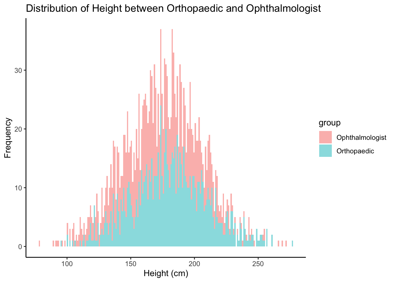
Most research needs to have a research question, which means you have to have a hypothesis to test and sufficient data to demonstrate whether to accept or reject your hypothesis.
An effective research question must include:
An outcome measure (e.g., weight, height, success, failure, pain score, anxiety score)
An exposure or intervention (e.g., surgery, time, diagnosis, treatment)
An idea of the direction and magnitude of the difference between the groups (e.g., higher, lower, different)
For example, a simple research question might be:
To determine whether the height (outcome) between orthopaedic surgeons and ophthalmologists (exposure: type of specialty) differs by 10cm (magnitude of difference).
The null hypothesis (H₀) represents the status quo or the assumption of no difference. To show that there is a difference, you must disprove H₀.
By disproving H₀, you support H₁.
A simplified formula for the sample size required for detecting a difference between two means (or continuous variables) is:
\[ n = \frac{\left(Z_{1-\alpha/2} + Z_{1-\beta}\right)^2 \, \sigma^2}{\Delta^2} \]
We need to fill in some values with our best guesses, or info from exisitng literature.
Where:
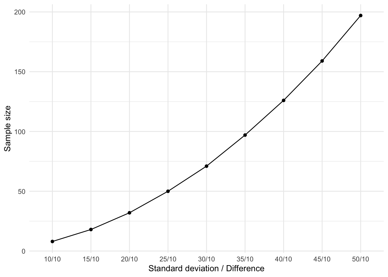
In normal language: We want to show atleast the \(\Delta\) between the two groups. I like to call \(\Delta\) the minimum detectable difference - If the actual difference is smaller than 10cm, we will not be able to detect it.
You must also consider the variability in each group. In other words each persons height will vary, or is spread around the mean. We describe this by the standard deviation (SD) (σ) of the outcome. As a sample size increases, the SD becomes narrower.
SD is calculated by taking the square root of the differences between each value and the mean, squaring them, summing them, and dividing by the number of values.
[1] 12.5
     Two-sample t test power calculation

              n = 142.2462
              d = 0.3333333
      sig.level = 0.05
          power = 0.8
    alternative = two.sided

NOTE: n is number in *each* group
Finding a difference that is equal to the to or more than the standard deviation is ideal but this is generally not the case in real life, often you may wish to find a smaller difference with a much larger spread of data around a mean. Remember spread (or variance) can be affect by the natural variablitly of the event you are observing or the measurement process itself. Think of how much variation you see in the measuremnts you observe each day, from patietns weight, CD4 count, blood pressure, etc.
Research Question: To determine whether the height between orthopaedic surgeons and ophthalmologists differs by 10cm.
Null Hypothesis: The heights are not different by more than 10cm between the two groups.
A p-value of <0.05 means we reject the null hypothesis and accept the alternative hypothesis.
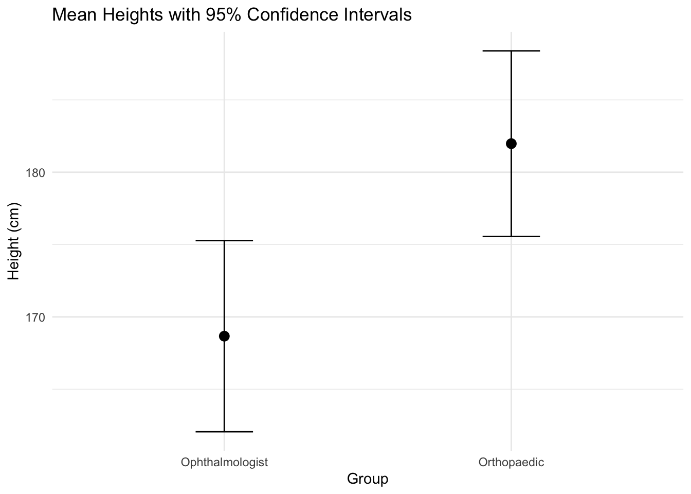
We determined the sample size by calculating the number of participants needed to detect a difference of 10 cm with a power of 80% and a significance level of 5%. Both groups had a standard deviation of 15 cm. This results in a sample size of 142 (or 71 per group).
| Characteristic | Ophthalmologist N = 71 (95% CI)1 |
Orthopaedic N = 71 (95% CI)1 |
p-value2 |
|---|---|---|---|
| height | 168 (28) (162, 175) | 182 (27) (175, 188) | 0.004 |
| Abbreviation: CI = Confidence Interval | |||
| 1 Mean (SD) | |||
| 2 Welch Two Sample t-test | |||